Designing an algorithm to compute the optimal set of BLAST hits

Problem

My problem is simple: given a set of BLAST results, how do I select the best set of mutually compatible high-scoring pairs? (A high-scoring pair is simply a hit between the query and subject sequences. It corresponds to an aligned portion of both, alongside an accompanying E value and bitscore indicating the quality of the hit.)

The above image demonstrates a simple example of the problem. The two HSPs are not mutually compatible–A precedes B in the query sequence, yet appears after it in the subject sequence. Our goal is to choose only the best subset of mutually compatible HSPs, where we take “best” to mean the subset of HSPs with the highest total bitscore. Resolving the problem in this instance is trivial–simply select A, discarding B, as A has a higher bitscore (stemming from its longer length relative to B).

What do we do, however, in more complex cases?

Here we have 14 HSPs exhibiting complex crossing and overlapping patterns. Choosing the subset that yields the highest summed bit score is considerably more difficult. To resolve this, I designed a dynamic programming algorithm that efficiently produces an optimal solution. Applied to the problem above, it yields the following:

I’m using this algorithm to compare two genomes for the parasitic nematode Haemonchus contortus. The two published genomes, genome A and genome B, differ substantially in their representation of the organism. Particularly curious is that, according to InParanoid, 60% of the annotated genes in genome A have no orthologue in genome B. Given that both genomes correspond to the same species, we’d expect their annotated genes to be nearly identical, and so this number should instead be at least 95%.

To investigate this phenomenon, I BLASTed the 16,000 missing genes from genome A against genome B, in an attempt to ascertain whether they were present in genome B’s assembly. If they were not, this was a clear case of misassembly. Given the 16,000 genes of interest, this approach required an automated means of scoring each according to how well it was represented in B’s assembly. While my Approach 1 below yielded an answer, a proper solution required a more complex algorithm that computed the optimal set of mutually compatible HSPs, which I describe in Approaches 2 and 3.

Approach 1: Compute union of BLAST HSPs

My first attempt at scoring each of my 16,000 genes according to how well they were represented in genome B was straightforward: I took the union of each HSP’s query portion, then determined how much of the query sequence this represented. Let’s return to my simple example.

In this case, the union of the HSPs’ query portions consists of [2, 8]∪[11,13], whose total length is 7 + 3 = 10 nt (due to the inclusive nature of BLAST’s coordinates). The query sequence as a whole is 17 nt. Thus, the score for this particular query/subject pair is 10/17 = 0.588. I would then compute this value for all query/subject pairs for the gene (query) in question, taking the highest as this gene’s score. When I did this for all 16,000 genes, however, I was taken aback.

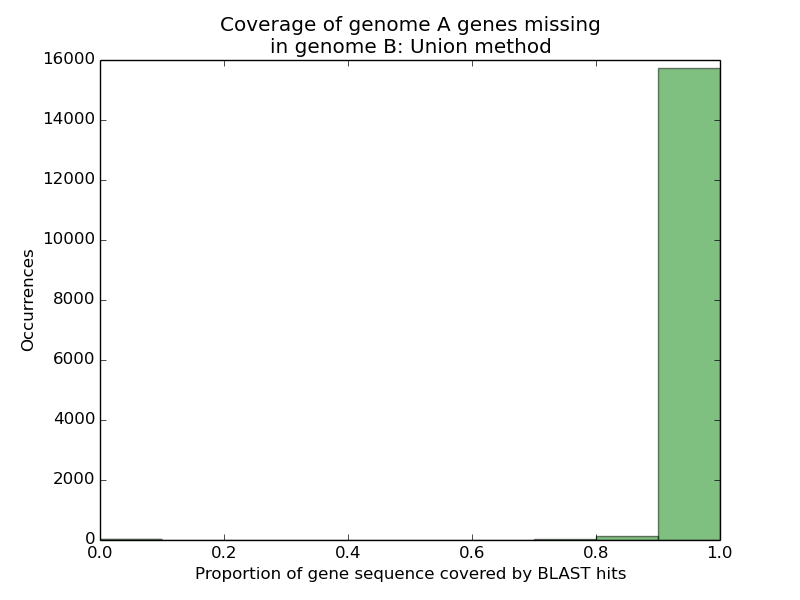
Almost all 16,000 missing genes from genome A had 90% or more of their sequences appearing on single scaffolds in genome B. Given that InParanoid could not find reasonable hits for any of these genes in genome B, this number was peculiar. Assuming genome A was accurate in annotating these genes, three possibilities arose:

1. Perhaps genome B’s annotation was really bad, even though its assembly was of reasonable quality. As InParanoid relies on the annotation, this could explain the missing orthologues in genome B.

2. Perhaps InParanoid was simply wrong. Bioinformatics’ golden rule is, after all, Thou shalt not trust thy tools.

3. Perhaps my methodology was not merely simple, but simplistic.

This last possibility seemed the most probable–as my algorithm simply took the union, it did not resolve cases where BLAST hits overlapped the same portion of the query or subject sequences, or where they “crossed” each other as in my first example above. With these caveats in mind, I set off in search of a better solution.

Approach 2: Choose best combination of mutually compatible BLAST HSPs

Clearly, evaluating a BLAST result’s quality by taking the union of query sequence intervals comprising it suffered from substantial limitations. Consequently, I decided to determine the optimal set of mutually compatible HSPs, which would neither overlap nor cross each other, on either their query or subject sequence portions.

My first attempt in this vein involved computing every possible combination of mutually compatible intervals, then scoring each according to how much of the query sequence it represented. In Python-flavoured pseudocode, my approach was thus. (All code is available in a non-pseudo, fully functioning version.)

def compute_combos_dumb(L):
  Sort L by query_start coordinates return
  compute_combos_dumb_r([], L)

def compute_combos_dumb_r(base, remaining):
  if len(remaining) == 0:
    return [base]
  first = remaining[0]
  rest = remaining[1:]

  if len(base) > 0:
    # Get query_end and subject_end for last interval in base
    base_query_end = base[-1].query_end
    base_subject_end = base[-1].subject_end
  else:
    # Nothing in base yet, so set to dummy values
    base_query_end = 0
    base_subject_end = 0

  if first.query_start > base_query_end and first.subject_start > base_subject_end:
    # If `first` is compatible with all the intervals in base, then we must
    # compute all combinations that include it (first call), and all
    # combinations that exclude it (second call).
    return compute_combos_dumb_r(base + [first], rest) + compute_combos_dumb_r(base, rest)
  else:
    # `first` is incompatible with something in base set, so only valid
    # combinations will be those that exclude it.
    return self._combo_r(base, rest)

At its heart, computing combinations relies on one rule: for a given set element E, one-half of all combinations will include E, while one-half won’t. This maxim lends itself to a straightforward recursive algorithm to compute all combinations. The code above implements this idea, but substantially cuts down the number of potential combinations–a given HSP is included in valid combinations only if it’s compatible with (meaning it doesn’t overlap or cross) all HSPs that precede it in the query (i.e., HSPs falling on lower query sequence coordinates).

When I tested this algorithm on a small data set, it worked wonderfully well. Alas, when I ran on the full data set, it ran overnight without producing anything of worth. As it relies on computing all combinations, it has exponential runtime–given n HSPs for a query/subject pair, there are 2ⁿ possible combinations of them. When I examined my data set in more detail, consisting of 16,000 genes, I found the most fecund featured some 114 HSPs, meaning there were 2¹¹⁴ possible combinations. While my algorithm cut down on this substantially by immediately rejecting any combinations with an HSP incompatible with those preceding it, not computing any additional combinations including it, this was insufficient to render my approach tractable.

Remember that I was only interested in the best set of mutually compatible HSPs–after computing all valid combinations, I scored each according to how much of the query sequence it represented, then threw away all others. As I wanted an answer some time before the heat death of the universe, I had to return to the drawing board.

Approach 3: Choose the best combination, but without taking exponential time

As I had already established a valid (though woefully inefficient) recursive algorithm for computing the best interval, a dynamic programming approach was natural. My method drew heavily on my previous approach–I simply ordered HSPs according to their position in the query sequence, then, starting at the last, recursively computed the optimal solution. For a given HSP H, two possible solutions existed:

1. We could include H in the solution. Then the optimal solution consisted of H, as well as the optimal solution for all HSPs preceding H that were also compatible with H (meaning they didn’t cross or overlap it).

2. We could exclude H from the solution. Then the optimal solution was merely the optimal solution for all HSPs preceding H.

Deciding which of these two approaches was best simply meant taking whichever of the two had the higher summed bitscore.

After mulling over the problem, I settled on a solution that, strictly speaking, is not an instance of dynamic programming. Dynamic programming usually requires you define a recursive solution in which the optimal solution to a problem is defined in terms of optimal subproblems, then pre-computing these smaller solutions before trying to solve the full one. Merely memoizing the recursive function (i.e., caching the output produced for a given input) allowed the algorithm to chew through all 16,000 query sequences in approximately ninety seconds, however, so I had no reason to pursue further optimization. The algorithm, then, was roughly thus:

# Return summed bitscores of best combo. To figure out which HSPs
# correspond to this optimal score, we must also store whether the optimal
# solution includes the last HSP in `hsps` at each step, then recursively
# reconstruct the optimal solution after the algorithm finishes. See the
# linked code for details.
def compute_combos_smart(hsps):
  # Memoize the function so that, if we have already computed the solution
  # for `hsps`, just fetch and return that value immediately without
  # performing below computations.

  if len(hsps) == 0:
    return 0
  if len(hsps) == 1:
    # Trivial solution: one HSP, so optimal solution is just itself.
    return hsps[0].bitscore

  # Last HSP
  last_hsp = hsps[-1]
  # All HSPs except last
  previous = hsps[:-1]

  # Find subset of HSPs in `previous` that don't overlap `last_hsp`.
  compatible = find_compatible(last_hsp, previous)

  best_without_last = compute_combos_smart(previous)
  best_with_last    = compute_combos_smart(compatible) + last_hsp.bitscore
  return max(best_without_last, best_with_last)

def find_compatible(target, hsps):
  '''Find hsps amongst `hsps` that don't overlap or cross `target`. They
  may not be mutually compatible, as they are only guaranteed to be
  compatible with `target`.'''
  compatible = []

  for hsp in hsps:
    # Don't define target as being compatible with itself.
    if hsp == target:
      continue

    if target.query_start <= hsp.query_start:
      first, second = target, hsp
    else:
      first, second = hsp, target

    overlap = second.query_start <= first.query_end or
              second.subject_start <= first.subject_end
    if not overlap:
      compatible.append(hsp)

return compatible

And, the result:

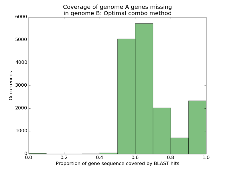
Observe that, unlike our earlier result, we now find a substantially worse representation of genome A’s missing genes in genome B’s assembly. When scoring genes according to how much of their sequence was recovered via mutually compatible HSPs, rather than the union of all HSPs, we see that only 14.7% of genes can have more than nine-tenths of their sequence recovered, versus the 98.8% we saw before.

I feel the need, the need, for speed

One further optimization remained. By partitioning HSPs into nonoverlapping sets, you can solve each partition separately.

Each of the two non-overlapping sets of HSPs in the above figure can be solved independently without impacting the optimality of the solution. Implementing this optimization had no effect on the runtime of the algorithm, however–the existing memoization of the recursive function made repeated queries concerning optimal values for HSPs that could form their own partitions extremely fast, so explicitly partitioning the data yielded no speed-up.

Conclusion

Dynamic programming makes choosing optimal sets of mutually compatible HSPs fun.

Post navigation